
0x00 前言
最近对数据科学有点感兴趣,众所周知,在 python 中用来做数据处理常用的有 numpy、pandas 等模块,它们功能非常强大。
考虑到有项目正好要用到 pandas,这次就来学一下吧。(挺久之前就想学的,一直咕
看到网上推荐了官方的 10 Minutes to pandas,就去看了一下,翻译了一下官方的教程,自己跑了代码,顺便再记了点笔记吧。
下面的内容主要参考的是10 Minutes to pandas(然而看了一晚上),运行环境为 Jupyter Notebook。
这篇博客也是在从 Jupyter Notebook 里导出的 markdown 基础上完成的,挺方便的呢。(有些地方可能由于博客样式的原因显示会有点问题,凑合着看一看吧。
后面有空再整理一下,放个 Jupyter Notebook 的.ipynb版本吧。
—->详见文末的更新!
0x01 导入模块
import pandas as pd
import matplotlib.pyplot as plt
import numpy as np
这些都是常用别名了呢(
0x02 创建对象 Object Creation
传递一个list对象来创建一个Series,pandas会默认创建整型索引(index)。
s = pd.Series([1,3,5,np.nan,6,8])
s
0 1.0
1 3.0
2 5.0
3 NaN
4 6.0
5 8.0
dtype: float64
传递一个numpy array,时间索引以及列标签来创建一个DataFrame
dates = pd.date_range('20200416', periods=6)
dates
DatetimeIndex(['2020-04-16', '2020-04-17', '2020-04-18', '2020-04-19',
'2020-04-20', '2020-04-21'],
dtype='datetime64[ns]', freq='D')
df = pd.DataFrame(np.random.randn(6,4), index=dates, columns=list('ABCD'))
df| A | B | C | D | |
|---|---|---|---|---|
| 2020-04-16 | -0.228084 | 0.712521 | 0.743378 | 0.526823 |
| 2020-04-17 | -0.423923 | 0.564346 | -2.318931 | 0.080931 |
| 2020-04-18 | -2.032243 | 2.046827 | 1.176614 | -0.365556 |
| 2020-04-19 | -1.200005 | 1.109991 | -1.527804 | 1.068642 |
| 2020-04-20 | -0.535031 | 1.351420 | 0.907865 | -1.074013 |
| 2020-04-21 | -0.614734 | 0.027143 | -0.420875 | -0.333819 |
传递一个能够被转换成类似序列结构的字典对象来创建一个DataFrame
df2 = pd.DataFrame({ 'A' : 1.,
 'B' : pd.Timestamp('20200416183800'),
 'C' : pd.Series(1,index=list(range(4)),dtype='float32'),
 'D' : np.array([3] * 4,dtype='int32'),
 'E' : pd.Categorical(["test","train","test","train"]),
 'F' : 'foo' })
df2| A | B | C | D | E | F | |
|---|---|---|---|---|---|---|
| 0 | 1.0 | 2020-04-16 18:38:00 | 1.0 | 3 | test | foo |
| 1 | 1.0 | 2020-04-16 18:38:00 | 1.0 | 3 | train | foo |
| 2 | 1.0 | 2020-04-16 18:38:00 | 1.0 | 3 | test | foo |
| 3 | 1.0 | 2020-04-16 18:38:00 | 1.0 | 3 | train | foo |
查看他们的数据类型(dtypes).
df2.dtypesA float64
B datetime64[ns]
C float32
D int32
E category
F object
dtype: object
在 IPython 里输入 df2.,按下 TAB 键,会有常用的代码提示。
这里我是在 Jupyter Notebook 中跑,也有类似效果。为了方便展示这里用dir来列出来吧。
dir(df2)['A',
'B',
'C',
'D',
'E',
'F',
'T',
######################...###########
'to_feather',
'to_gbq',
'to_hdf',
'to_html',
'to_json',
'to_latex',
'to_msgpack',
'to_numpy',
'to_panel',
'to_parquet',
'to_period',
'to_pickle',
'to_records',
'to_sparse',
'to_sql',
'to_stata',
'to_string',
'to_timestamp',
'to_xarray',
'transform',
'transpose',
'truediv',
'truncate',
'tshift',
'tz_convert',
'tz_localize',
'unstack',
'update',
'values',
'var',
'where',
'xs']
0x03 查看数据 Viewing Data
查看 frame 中头部和尾部的行
df.head() # 查看前五行数据| A | B | C | D | |
|---|---|---|---|---|
| 2020-04-16 | -0.228084 | 0.712521 | 0.743378 | 0.526823 |
| 2020-04-17 | -0.423923 | 0.564346 | -2.318931 | 0.080931 |
| 2020-04-18 | -2.032243 | 2.046827 | 1.176614 | -0.365556 |
| 2020-04-19 | -1.200005 | 1.109991 | -1.527804 | 1.068642 |
| 2020-04-20 | -0.535031 | 1.351420 | 0.907865 | -1.074013 |
df.head(2) # 前两行| A | B | C | D | |
|---|---|---|---|---|
| 2020-04-16 | -0.228084 | 0.712521 | 0.743378 | 0.526823 |
| 2020-04-17 | -0.423923 | 0.564346 | -2.318931 | 0.080931 |
df.tail(3) # 倒数三行| A | B | C | D | |
|---|---|---|---|---|
| 2020-04-19 | -1.200005 | 1.109991 | -1.527804 | 1.068642 |
| 2020-04-20 | -0.535031 | 1.351420 | 0.907865 | -1.074013 |
| 2020-04-21 | -0.614734 | 0.027143 | -0.420875 | -0.333819 |
显示索引、列和底层的(underlying) numpy 数据
df| A | B | C | D | |
|---|---|---|---|---|
| 2020-04-16 | -0.228084 | 0.712521 | 0.743378 | 0.526823 |
| 2020-04-17 | -0.423923 | 0.564346 | -2.318931 | 0.080931 |
| 2020-04-18 | -2.032243 | 2.046827 | 1.176614 | -0.365556 |
| 2020-04-19 | -1.200005 | 1.109991 | -1.527804 | 1.068642 |
| 2020-04-20 | -0.535031 | 1.351420 | 0.907865 | -1.074013 |
| 2020-04-21 | -0.614734 | 0.027143 | -0.420875 | -0.333819 |
df.indexDatetimeIndex(['2020-04-16', '2020-04-17', '2020-04-18', '2020-04-19',
'2020-04-20', '2020-04-21'],
dtype='datetime64[ns]', freq='D')
df2.indexInt64Index([0, 1, 2, 3], dtype='int64')
df.columnsIndex(['A', 'B', 'C', 'D'], dtype='object')
df.valuesarray([[-0.22808386, 0.71252123, 0.74337822, 0.52682341],
[-0.42392275, 0.56434629, -2.31893066, 0.08093058],
[-2.03224294, 2.04682736, 1.17661398, -0.3655562 ],
[-1.20000469, 1.10999124, -1.52780407, 1.06864157],
[-0.53503099, 1.35142044, 0.90786509, -1.07401348],
[-0.61473412, 0.02714293, -0.42087502, -0.33381946]])
df2.valuesarray([[1.0, Timestamp('2020-04-16 18:38:00'), 1.0, 3, 'test', 'foo'],
[1.0, Timestamp('2020-04-16 18:38:00'), 1.0, 3, 'train', 'foo'],
[1.0, Timestamp('2020-04-16 18:38:00'), 1.0, 3, 'test', 'foo'],
[1.0, Timestamp('2020-04-16 18:38:00'), 1.0, 3, 'train', 'foo']],
dtype=object)
print(type(df))
print(type(df.columns))
print(type(df.values))
<class 'pandas.core.frame.DataFrame'>
<class 'pandas.core.indexes.base.Index'>
<class 'numpy.ndarray'>
describe 函数对于数据的快速统计汇总
df.describe()| A | B | C | D | |
|---|---|---|---|---|
| count | 6.000000 | 6.000000 | 6.000000 | 6.000000 |
| mean | -0.839003 | 0.968708 | -0.239959 | -0.016166 |
| std | 0.669679 | 0.699208 | 1.435586 | 0.751411 |
| min | -2.032243 | 0.027143 | -2.318931 | -1.074013 |
| 25% | -1.053687 | 0.601390 | -1.251072 | -0.357622 |
| 50% | -0.574883 | 0.911256 | 0.161252 | -0.126444 |
| 75% | -0.451700 | 1.291063 | 0.866743 | 0.415350 |
| max | -0.228084 | 2.046827 | 1.176614 | 1.068642 |
df2.describe()| A | C | D | |
|---|---|---|---|
| count | 4.0 | 4.0 | 4.0 |
| mean | 1.0 | 1.0 | 3.0 |
| std | 0.0 | 0.0 | 0.0 |
| min | 1.0 | 1.0 | 3.0 |
| 25% | 1.0 | 1.0 | 3.0 |
| 50% | 1.0 | 1.0 | 3.0 |
| 75% | 1.0 | 1.0 | 3.0 |
| max | 1.0 | 1.0 | 3.0 |
对数据进行转置(Transposing)
df.T| 2020-04-16 00:00:00 | 2020-04-17 00:00:00 | 2020-04-18 00:00:00 | 2020-04-19 00:00:00 | 2020-04-20 00:00:00 | 2020-04-21 00:00:00 | |
|---|---|---|---|---|---|---|
| A | -0.228084 | -0.423923 | -2.032243 | -1.200005 | -0.535031 | -0.614734 |
| B | 0.712521 | 0.564346 | 2.046827 | 1.109991 | 1.351420 | 0.027143 |
| C | 0.743378 | -2.318931 | 1.176614 | -1.527804 | 0.907865 | -0.420875 |
| D | 0.526823 | 0.080931 | -0.365556 | 1.068642 | -1.074013 | -0.333819 |
df2.T| 0 | 1 | 2 | 3 | |
|---|---|---|---|---|
| A | 1 | 1 | 1 | 1 |
| B | 2020-04-16 18:38:00 | 2020-04-16 18:38:00 | 2020-04-16 18:38:00 | 2020-04-16 18:38:00 |
| C | 1 | 1 | 1 | 1 |
| D | 3 | 3 | 3 | 3 |
| E | test | train | test | train |
| F | foo | foo | foo | foo |
按照某一坐标轴进行排序
df.sort_index(axis=1, ascending=False) # 降序| D | C | B | A | |
|---|---|---|---|---|
| 2020-04-16 | 0.526823 | 0.743378 | 0.712521 | -0.228084 |
| 2020-04-17 | 0.080931 | -2.318931 | 0.564346 | -0.423923 |
| 2020-04-18 | -0.365556 | 1.176614 | 2.046827 | -2.032243 |
| 2020-04-19 | 1.068642 | -1.527804 | 1.109991 | -1.200005 |
| 2020-04-20 | -1.074013 | 0.907865 | 1.351420 | -0.535031 |
| 2020-04-21 | -0.333819 | -0.420875 | 0.027143 | -0.614734 |
df.sort_index(axis=1, ascending=True) # 升序(默认)| A | B | C | D | |
|---|---|---|---|---|
| 2020-04-16 | -0.228084 | 0.712521 | 0.743378 | 0.526823 |
| 2020-04-17 | -0.423923 | 0.564346 | -2.318931 | 0.080931 |
| 2020-04-18 | -2.032243 | 2.046827 | 1.176614 | -0.365556 |
| 2020-04-19 | -1.200005 | 1.109991 | -1.527804 | 1.068642 |
| 2020-04-20 | -0.535031 | 1.351420 | 0.907865 | -1.074013 |
| 2020-04-21 | -0.614734 | 0.027143 | -0.420875 | -0.333819 |
df.sort_index(axis=0, ascending=False) # 以第0轴(行)来排序,降序| A | B | C | D | |
|---|---|---|---|---|
| 2020-04-21 | -0.614734 | 0.027143 | -0.420875 | -0.333819 |
| 2020-04-20 | -0.535031 | 1.351420 | 0.907865 | -1.074013 |
| 2020-04-19 | -1.200005 | 1.109991 | -1.527804 | 1.068642 |
| 2020-04-18 | -2.032243 | 2.046827 | 1.176614 | -0.365556 |
| 2020-04-17 | -0.423923 | 0.564346 | -2.318931 | 0.080931 |
| 2020-04-16 | -0.228084 | 0.712521 | 0.743378 | 0.526823 |
按值进行排序,默认为升序
df.sort_values(by='B')| A | B | C | D | |
|---|---|---|---|---|
| 2020-04-21 | -0.614734 | 0.027143 | -0.420875 | -0.333819 |
| 2020-04-17 | -0.423923 | 0.564346 | -2.318931 | 0.080931 |
| 2020-04-16 | -0.228084 | 0.712521 | 0.743378 | 0.526823 |
| 2020-04-19 | -1.200005 | 1.109991 | -1.527804 | 1.068642 |
| 2020-04-20 | -0.535031 | 1.351420 | 0.907865 | -1.074013 |
| 2020-04-18 | -2.032243 | 2.046827 | 1.176614 | -0.365556 |
0x04 选择数据 Selection
注意: 虽然标准的 Python/Numpy 的选择和设置表达式都非常易懂且方便用于交互使用,但是作为工程使用的代码,推荐使用经过优化的 pandas 数据访问方法:
.at,.iat,.loc,.iloc和.ix。
0x04-1 获取 Getting
选择一个单独的列,这将会返回一个 Series,等效于 df.A
df['A']2020-04-16 -0.228084
2020-04-17 -0.423923
2020-04-18 -2.032243
2020-04-19 -1.200005
2020-04-20 -0.535031
2020-04-21 -0.614734
Freq: D, Name: A, dtype: float64
通过[]进行选择,可以用来行进行切片(slice)
df[1:3]| A | B | C | D | |
|---|---|---|---|---|
| 2020-04-17 | -0.423923 | 0.564346 | -2.318931 | 0.080931 |
| 2020-04-18 | -2.032243 | 2.046827 | 1.176614 | -0.365556 |
df['20200418':'20200420']| A | B | C | D | |
|---|---|---|---|---|
| 2020-04-18 | -2.032243 | 2.046827 | 1.176614 | -0.365556 |
| 2020-04-19 | -1.200005 | 1.109991 | -1.527804 | 1.068642 |
| 2020-04-20 | -0.535031 | 1.351420 | 0.907865 | -1.074013 |
0x4-2 通过标签选择 Selection by Label
利用 pandas 的 .loc, .at 方法
使用标签来获取一个交叉的区域
dates[0]Timestamp('2020-04-16 00:00:00', freq='D')
df.loc[dates[0]]A -0.228084
B 0.712521
C 0.743378
D 0.526823
Name: 2020-04-16 00:00:00, dtype: float64
用标签来在多个轴上进行选择
df.loc[:,['A','B']]| A | B | |
|---|---|---|
| 2020-04-16 | -0.228084 | 0.712521 |
| 2020-04-17 | -0.423923 | 0.564346 |
| 2020-04-18 | -2.032243 | 2.046827 |
| 2020-04-19 | -1.200005 | 1.109991 |
| 2020-04-20 | -0.535031 | 1.351420 |
| 2020-04-21 | -0.614734 | 0.027143 |
利用标签来切片
注意此处的切片两端都包含(左闭右闭)
df.loc['20200418':'20200420',['A','B']]| A | B | |
|---|---|---|
| 2020-04-18 | -2.032243 | 2.046827 |
| 2020-04-19 | -1.200005 | 1.109991 |
| 2020-04-20 | -0.535031 | 1.351420 |
df.loc[dates[2]:,:'C']| A | B | C | |
|---|---|---|---|
| 2020-04-18 | -2.032243 | 2.046827 | 1.176614 |
| 2020-04-19 | -1.200005 | 1.109991 | -1.527804 |
| 2020-04-20 | -0.535031 | 1.351420 | 0.907865 |
| 2020-04-21 | -0.614734 | 0.027143 | -0.420875 |
对于返回的对象进行维度缩减
df.loc['20200419',['A','B']]A -1.200005
B 1.109991
Name: 2020-04-19 00:00:00, dtype: float64
获取一个标量
df.loc[dates[2],'A']-2.0322429408627056
快速访问一个标量(与上一个方法等价)
df.at[dates[2],'A']-2.0322429408627056
0x04-3 通过位置进行选择 Selection by Position
利用的是 pandas 里的 .iloc, .iat 方法
通过传递整数值进行位置选择
df.iloc[3] A -1.200005
B 1.109991
C -1.527804
D 1.068642
Name: 2020-04-19 00:00:00, dtype: float64
df.iloc[:,2] # [行,列] 或 [第0维,第1维]2020-04-16 0.743378
2020-04-17 -2.318931
2020-04-18 1.176614
2020-04-19 -1.527804
2020-04-20 0.907865
2020-04-21 -0.420875
Freq: D, Name: C, dtype: float64
利用数值进行切片,类似于 numpy/python
注意一下,这里的切片是普通的切片,即左闭右开。
df.iloc[3:5,0:2]| A | B | |
|---|---|---|
| 2020-04-19 | -1.200005 | 1.109991 |
| 2020-04-20 | -0.535031 | 1.351420 |
可以指定一个位置的列表来选择数据区域
df.iloc[[1,2,4],[0,2]]| A | C | |
|---|---|---|
| 2020-04-17 | -0.423923 | -2.318931 |
| 2020-04-18 | -2.032243 | 1.176614 |
| 2020-04-20 | -0.535031 | 0.907865 |
对行进行切片
df.iloc[1:3,:]| A | B | C | D | |
|---|---|---|---|---|
| 2020-04-17 | -0.423923 | 0.564346 | -2.318931 | 0.080931 |
| 2020-04-18 | -2.032243 | 2.046827 | 1.176614 | -0.365556 |
对列进行切片
df.iloc[:,1:3]| B | C | |
|---|---|---|
| 2020-04-16 | 0.712521 | 0.743378 |
| 2020-04-17 | 0.564346 | -2.318931 |
| 2020-04-18 | 2.046827 | 1.176614 |
| 2020-04-19 | 1.109991 | -1.527804 |
| 2020-04-20 | 1.351420 | 0.907865 |
| 2020-04-21 | 0.027143 | -0.420875 |
利用位置快速得到一个位置对应的值
df.iloc[1,1]0.5643462917985026
df.iat[1,1]0.5643462917985026
.ix 用法(Deprecated)
df.ix[] 既可以通过整数索引进行数据选取,也可以通过标签索引进行数据选取。
也就是说,df.ix[] 是 df.loc[] 和 df.iloc[] 的功能集合,且在同义词选取中,可以同时使用整数索引和标签索引。
这个方法在官方的 10 Minutes to pandas 中没有专门说明,不建议用这一方法,请用.loc和.iloc来索引,那这里就提一下好了。
df.ix[1,'A']D:\Programs\Anaconda\lib\site-packages\ipykernel_launcher.py:1: DeprecationWarning:
.ix is deprecated. Please use
.loc for label based indexing or
.iloc for positional indexing
See the documentation here:
http://pandas.pydata.org/pandas-docs/stable/indexing.html#ix-indexer-is-deprecated
"""Entry point for launching an IPython kernel.
-1.363418018143355
df.ix[dates[1:3],[0,2,3]]D:\Programs\Anaconda\lib\site-packages\ipykernel_launcher.py:1: DeprecationWarning:
.ix is deprecated. Please use
.loc for label based indexing or
.iloc for positional indexing
See the documentation here:
http://pandas.pydata.org/pandas-docs/stable/indexing.html#ix-indexer-is-deprecated
"""Entry point for launching an IPython kernel.
| A | C | D | |
|---|---|---|---|
| 2020-04-17 | -11.332834 | 7.659436 | -20.925183 |
| 2020-04-18 | -11.040688 | 6.867701 | -20.157355 |
从 DeprecationWarning 看来的确已经 deprecated 了,那就不要用了!
0x04-4 布尔索引 Boolean Indexing
使用一个单独列的值来选择数据
df[df.D > 0]| A | B | C | D | |
|---|---|---|---|---|
| 2020-04-16 | -0.228084 | 0.712521 | 0.743378 | 0.526823 |
| 2020-04-17 | -0.423923 | 0.564346 | -2.318931 | 0.080931 |
| 2020-04-19 | -1.200005 | 1.109991 | -1.527804 | 1.068642 |
利用布尔条件从一个 DataFrame 中选择数据
df>0| A | B | C | D | |
|---|---|---|---|---|
| 2020-04-16 | False | True | True | True |
| 2020-04-17 | False | True | False | True |
| 2020-04-18 | False | True | True | False |
| 2020-04-19 | False | True | False | True |
| 2020-04-20 | False | True | True | False |
| 2020-04-21 | False | True | False | False |
df[df > 0]| A | B | C | D | |
|---|---|---|---|---|
| 2020-04-16 | NaN | 0.712521 | 0.743378 | 0.526823 |
| 2020-04-17 | NaN | 0.564346 | NaN | 0.080931 |
| 2020-04-18 | NaN | 2.046827 | 1.176614 | NaN |
| 2020-04-19 | NaN | 1.109991 | NaN | 1.068642 |
| 2020-04-20 | NaN | 1.351420 | 0.907865 | NaN |
| 2020-04-21 | NaN | 0.027143 | NaN | NaN |
使用 isin() 方法来过滤数据
(is in)
df3 = df.copy()
df3['E'] = ['one', 'one','two','three','four','three']
df3| A | B | C | D | E | |
|---|---|---|---|---|---|
| 2020-04-16 | -0.228084 | 0.712521 | 0.743378 | 0.526823 | one |
| 2020-04-17 | -0.423923 | 0.564346 | -2.318931 | 0.080931 | one |
| 2020-04-18 | -2.032243 | 2.046827 | 1.176614 | -0.365556 | two |
| 2020-04-19 | -1.200005 | 1.109991 | -1.527804 | 1.068642 | three |
| 2020-04-20 | -0.535031 | 1.351420 | 0.907865 | -1.074013 | four |
| 2020-04-21 | -0.614734 | 0.027143 | -0.420875 | -0.333819 | three |
df3[df3['E'].isin(['two','four'])]| A | B | C | D | E | |
|---|---|---|---|---|---|
| 2020-04-18 | -2.032243 | 2.046827 | 1.176614 | -0.365556 | two |
| 2020-04-20 | -0.535031 | 1.351420 | 0.907865 | -1.074013 | four |
0x05 设置数据 Setting
设置一个新的列,自动按照索引来对其数据
s1 = pd.Series([1,2,3,4,5,6], index=pd.date_range('20200416', periods=6))
s1
2020-04-16 1
2020-04-17 2
2020-04-18 3
2020-04-19 4
2020-04-20 5
2020-04-21 6
Freq: D, dtype: int64
df['F'] = s1通过标签设置新的值
df.at[dates[0],'A'] = 0通过标签设置新的值
df.iat[0,1] = 0通过一个 numpy 数组设置一组新值
df.loc[:,'D'] = np.array([5] * len(df))上述操作结果如下
df| A | B | C | D | F | |
|---|---|---|---|---|---|
| 2020-04-16 | 0.000000 | 0.000000 | 0.743378 | 5 | 1 |
| 2020-04-17 | -0.423923 | 0.564346 | -2.318931 | 5 | 2 |
| 2020-04-18 | -2.032243 | 2.046827 | 1.176614 | 5 | 3 |
| 2020-04-19 | -1.200005 | 1.109991 | -1.527804 | 5 | 4 |
| 2020-04-20 | -0.535031 | 1.351420 | 0.907865 | 5 | 5 |
| 2020-04-21 | -0.614734 | 0.027143 | -0.420875 | 5 | 6 |
通过 where 操作来设置新的值
df2 = df.copy()
df2[df2 > 0] = -df2
df2| A | B | C | D | F | |
|---|---|---|---|---|---|
| 2020-04-16 | 0.000000 | 0.000000 | -0.743378 | -5 | -1 |
| 2020-04-17 | -0.423923 | -0.564346 | -2.318931 | -5 | -2 |
| 2020-04-18 | -2.032243 | -2.046827 | -1.176614 | -5 | -3 |
| 2020-04-19 | -1.200005 | -1.109991 | -1.527804 | -5 | -4 |
| 2020-04-20 | -0.535031 | -1.351420 | -0.907865 | -5 | -5 |
| 2020-04-21 | -0.614734 | -0.027143 | -0.420875 | -5 | -6 |
0x06 缺失值处理 Missing Data
在pandas中,使用np.nan来代替缺失值,这些值将默认不会包含在计算中。
reindex()方法可以对指定轴上的索引进行改变/增加/删除操作,返回原始数据的一个拷贝。
df1 = df.reindex(index=dates[0:4], columns=list(df.columns) + ['E'])
df1| A | B | C | D | F | E | |
|---|---|---|---|---|---|---|
| 2020-04-16 | 0.000000 | 0.000000 | 0.743378 | 5 | 1 | NaN |
| 2020-04-17 | -0.423923 | 0.564346 | -2.318931 | 5 | 2 | NaN |
| 2020-04-18 | -2.032243 | 2.046827 | 1.176614 | 5 | 3 | NaN |
| 2020-04-19 | -1.200005 | 1.109991 | -1.527804 | 5 | 4 | NaN |
df1.loc[dates[0]:dates[1],'E'] = 1
df1| A | B | C | D | F | E | |
|---|---|---|---|---|---|---|
| 2020-04-16 | 0.000000 | 0.000000 | 0.743378 | 5 | 1 | 1.0 |
| 2020-04-17 | -0.423923 | 0.564346 | -2.318931 | 5 | 2 | 1.0 |
| 2020-04-18 | -2.032243 | 2.046827 | 1.176614 | 5 | 3 | NaN |
| 2020-04-19 | -1.200005 | 1.109991 | -1.527804 | 5 | 4 | NaN |
去掉包含缺失值的行
df1.dropna(how='any')| A | B | C | D | F | E | |
|---|---|---|---|---|---|---|
| 2020-04-16 | 0.000000 | 0.000000 | 0.743378 | 5 | 1 | 1.0 |
| 2020-04-17 | -0.423923 | 0.564346 | -2.318931 | 5 | 2 | 1.0 |
填充缺失的值,利用value来指定
print(df1)
df1.fillna(value=5)
A B C D F E
2020-04-16 0.000000 0.000000 0.743378 5 1 1.0
2020-04-17 -0.423923 0.564346 -2.318931 5 2 1.0
2020-04-18 -2.032243 2.046827 1.176614 5 3 NaN
2020-04-19 -1.200005 1.109991 -1.527804 5 4 NaN
| A | B | C | D | F | E | |
|---|---|---|---|---|---|---|
| 2020-04-16 | 0.000000 | 0.000000 | 0.743378 | 5 | 1 | 1.0 |
| 2020-04-17 | -0.423923 | 0.564346 | -2.318931 | 5 | 2 | 1.0 |
| 2020-04-18 | -2.032243 | 2.046827 | 1.176614 | 5 | 3 | 5.0 |
| 2020-04-19 | -1.200005 | 1.109991 | -1.527804 | 5 | 4 | 5.0 |
获取值为nan的布尔值(boolean mask)
pd.isna(df1)| A | B | C | D | F | E | |
|---|---|---|---|---|---|---|
| 2020-04-16 | False | False | False | False | False | False |
| 2020-04-17 | False | False | False | False | False | False |
| 2020-04-18 | False | False | False | False | False | True |
| 2020-04-19 | False | False | False | False | False | True |
0x07 一些常用的操作 Operations
0x07-1 统计 Stats
这些操作不包括缺失数据
执行描述性统计:
df.mean() # 均值,默认为列的A -0.800989
B 0.849955
C -0.239959
D 5.000000
F 3.500000
dtype: float64
df.mean(1) # 指定坐标轴(此处为行)2020-04-16 1.348676
2020-04-17 0.964299
2020-04-18 1.838240
2020-04-19 1.476436
2020-04-20 2.344851
2020-04-21 1.998307
Freq: D, dtype: float64
对于拥有不同维度,需要对齐对象再进行操作。
Pandas 会自动的沿着指定的维度进行广播。
s = pd.Series([1,3,5,np.nan,6,8], index=dates).shift(2)
s
2020-04-16 NaN
2020-04-17 NaN
2020-04-18 1.0
2020-04-19 3.0
2020-04-20 5.0
2020-04-21 NaN
Freq: D, dtype: float64
print(df)
df.sub(s, axis='index')  # df-s
A B C D F
2020-04-16 0.000000 0.000000 0.743378 5 1
2020-04-17 -0.423923 0.564346 -2.318931 5 2
2020-04-18 -2.032243 2.046827 1.176614 5 3
2020-04-19 -1.200005 1.109991 -1.527804 5 4
2020-04-20 -0.535031 1.351420 0.907865 5 5
2020-04-21 -0.614734 0.027143 -0.420875 5 6
| A | B | C | D | F | |
|---|---|---|---|---|---|
| 2020-04-16 | NaN | NaN | NaN | NaN | NaN |
| 2020-04-17 | NaN | NaN | NaN | NaN | NaN |
| 2020-04-18 | -3.032243 | 1.046827 | 0.176614 | 4.0 | 2.0 |
| 2020-04-19 | -4.200005 | -1.890009 | -4.527804 | 2.0 | 1.0 |
| 2020-04-20 | -5.535031 | -3.648580 | -4.092135 | 0.0 | 0.0 |
| 2020-04-21 | NaN | NaN | NaN | NaN | NaN |
0x07-2 应用方法到数据 Apply
Applying functions to the data
df.apply(np.cumsum) # cumsum 默认按照行累加| A | B | C | D | F | |
|---|---|---|---|---|---|
| 2020-04-16 | 0.000000 | 0.000000 | 0.743378 | 5 | 1 |
| 2020-04-17 | -0.423923 | 0.564346 | -1.575552 | 10 | 3 |
| 2020-04-18 | -2.456166 | 2.611174 | -0.398938 | 15 | 6 |
| 2020-04-19 | -3.656170 | 3.721165 | -1.926743 | 20 | 10 |
| 2020-04-20 | -4.191201 | 5.072585 | -1.018877 | 25 | 15 |
| 2020-04-21 | -4.805935 | 5.099728 | -1.439752 | 30 | 21 |
df.apply(np.cumsum,axis=1) # 指定 cumsum 的 axis 参数,按照列累加| A | B | C | D | F | |
|---|---|---|---|---|---|
| 2020-04-16 | 0.000000 | 0.000000 | 0.743378 | 5.743378 | 6.743378 |
| 2020-04-17 | -0.423923 | 0.140424 | -2.178507 | 2.821493 | 4.821493 |
| 2020-04-18 | -2.032243 | 0.014584 | 1.191198 | 6.191198 | 9.191198 |
| 2020-04-19 | -1.200005 | -0.090013 | -1.617818 | 3.382182 | 7.382182 |
| 2020-04-20 | -0.535031 | 0.816389 | 1.724255 | 6.724255 | 11.724255 |
| 2020-04-21 | -0.614734 | -0.587591 | -1.008466 | 3.991534 | 9.991534 |
df.apply(lambda x: x.max() - x.min())A 2.032243
B 2.046827
C 3.495545
D 0.000000
F 5.000000
dtype: float64
0x07-3 直方图 Histogramming
s = pd.Series(np.random.randint(0, 7, size=10))
s
0 0
1 4
2 5
3 0
4 3
5 2
6 2
7 0
8 5
9 1
dtype: int32
s.value_counts()0 3
5 2
2 2
4 1
3 1
1 1
dtype: int64
0x07-4 字符串方法 String Methods
Series 在str属性中准备了一组字符串处理方法,可以方便地对数组的每个元素进行操作,如下面的代码片段所示。
注意str中的模式匹配通常默认使用’正则表达式(在某些情况下总是使用它们)。
s = pd.Series(['A', 'B', 'C', 'Aaba', 'Baca', np.nan, 'CABA', 'dog', 'cat'])
s.str.lower()
0 a
1 b
2 c
3 aaba
4 baca
5 NaN
6 caba
7 dog
8 cat
dtype: object
0x08 合并 Merge
pandas 提供了一系列的方法,在 join/merge 操作中,可以轻松地对Series, DataFrame和Panel对象进行各种集合逻辑以及关系代数的操作。
0x08-1 Concat
df = pd.DataFrame(np.random.randn(10, 4))
df| 0 | 1 | 2 | 3 | |
|---|---|---|---|---|
| 0 | -0.089143 | 0.087569 | 0.218078 | -0.336815 |
| 1 | -0.694835 | 0.108324 | -1.882762 | -0.220210 |
| 2 | -2.069784 | -0.788424 | -1.694595 | 0.569263 |
| 3 | 2.433036 | 0.719851 | -0.109935 | 0.177864 |
| 4 | -0.838252 | 1.117676 | 0.880839 | -1.118529 |
| 5 | 1.706060 | 0.290877 | -0.907941 | -0.532450 |
| 6 | 0.118169 | -0.496975 | -0.190422 | 0.783875 |
| 7 | -1.213645 | -0.489622 | -0.798443 | -0.471611 |
| 8 | -0.314598 | -2.658906 | -1.139778 | 0.374437 |
| 9 | 0.229281 | -1.372309 | 0.996916 | -1.013462 |
# break it into pieces
pieces = [df[:3], df[3:7], df[7:]]
pieces
[ 0 1 2 3
0 -0.089143 0.087569 0.218078 -0.336815
1 -0.694835 0.108324 -1.882762 -0.220210
2 -2.069784 -0.788424 -1.694595 0.569263,
0 1 2 3
3 2.433036 0.719851 -0.109935 0.177864
4 -0.838252 1.117676 0.880839 -1.118529
5 1.706060 0.290877 -0.907941 -0.532450
6 0.118169 -0.496975 -0.190422 0.783875,
0 1 2 3
7 -1.213645 -0.489622 -0.798443 -0.471611
8 -0.314598 -2.658906 -1.139778 0.374437
9 0.229281 -1.372309 0.996916 -1.013462]
pd.concat(pieces)| 0 | 1 | 2 | 3 | |
|---|---|---|---|---|
| 0 | -0.089143 | 0.087569 | 0.218078 | -0.336815 |
| 1 | -0.694835 | 0.108324 | -1.882762 | -0.220210 |
| 2 | -2.069784 | -0.788424 | -1.694595 | 0.569263 |
| 3 | 2.433036 | 0.719851 | -0.109935 | 0.177864 |
| 4 | -0.838252 | 1.117676 | 0.880839 | -1.118529 |
| 5 | 1.706060 | 0.290877 | -0.907941 | -0.532450 |
| 6 | 0.118169 | -0.496975 | -0.190422 | 0.783875 |
| 7 | -1.213645 | -0.489622 | -0.798443 | -0.471611 |
| 8 | -0.314598 | -2.658906 | -1.139778 | 0.374437 |
| 9 | 0.229281 | -1.372309 | 0.996916 | -1.013462 |
0x08-2 Join
类似于 SQL 类型的合并。
下面是 key 相同的情况。
left = pd.DataFrame({'key': ['foo', 'foo'], 'lval': [1, 2]})
left| key | lval | |
|---|---|---|
| 0 | foo | 1 |
| 1 | foo | 2 |
right = pd.DataFrame({'key': ['foo', 'foo'], 'rval': [4, 5]})
right| key | rval | |
|---|---|---|
| 0 | foo | 4 |
| 1 | foo | 5 |
pd.merge(left, right, on='key')| key | lval | rval | |
|---|---|---|---|
| 0 | foo | 1 | 4 |
| 1 | foo | 1 | 5 |
| 2 | foo | 2 | 4 |
| 3 | foo | 2 | 5 |
另一个例子,key 不同的情况。
left = pd.DataFrame({'key': ['foo', 'bar'], 'lval': [1, 2]})
left| key | lval | |
|---|---|---|
| 0 | foo | 1 |
| 1 | bar | 2 |
right = pd.DataFrame({'key': ['foo', 'bar'], 'rval': [4, 5]})
right| key | rval | |
|---|---|---|
| 0 | foo | 4 |
| 1 | bar | 5 |
pd.merge(left, right, on='key')| key | lval | rval | |
|---|---|---|---|
| 0 | foo | 1 | 4 |
| 1 | bar | 2 | 5 |
0x08-3 Append
将一行加入到一个 DataFrame 上
df = pd.DataFrame(np.random.randn(8, 4), columns=['A','B','C','D'])
df| A | B | C | D | |
|---|---|---|---|---|
| 0 | -2.727829 | -1.382168 | 0.961920 | 0.083472 |
| 1 | -0.297131 | -0.294723 | 0.303267 | -0.539177 |
| 2 | -0.226735 | -2.157170 | 1.559418 | 0.102023 |
| 3 | 0.569927 | -0.800855 | 0.918515 | 1.630873 |
| 4 | 0.402999 | -2.238052 | 2.181635 | 1.950669 |
| 5 | 1.238971 | -0.165159 | 0.688200 | 0.793499 |
| 6 | 1.356265 | -0.034859 | -0.020774 | 0.485487 |
| 7 | -1.793398 | 0.900625 | 0.365789 | -2.089145 |
s = df.iloc[3]
df.append(s, ignore_index=True) # 忽略 index| A | B | C | D | |
|---|---|---|---|---|
| 0 | -2.727829 | -1.382168 | 0.961920 | 0.083472 |
| 1 | -0.297131 | -0.294723 | 0.303267 | -0.539177 |
| 2 | -0.226735 | -2.157170 | 1.559418 | 0.102023 |
| 3 | 0.569927 | -0.800855 | 0.918515 | 1.630873 |
| 4 | 0.402999 | -2.238052 | 2.181635 | 1.950669 |
| 5 | 1.238971 | -0.165159 | 0.688200 | 0.793499 |
| 6 | 1.356265 | -0.034859 | -0.020774 | 0.485487 |
| 7 | -1.793398 | 0.900625 | 0.365789 | -2.089145 |
| 8 | 0.569927 | -0.800855 | 0.918515 | 1.630873 |
s = df.iloc[4]
df.append(s, ignore_index=False)| A | B | C | D | |
|---|---|---|---|---|
| 0 | -2.727829 | -1.382168 | 0.961920 | 0.083472 |
| 1 | -0.297131 | -0.294723 | 0.303267 | -0.539177 |
| 2 | -0.226735 | -2.157170 | 1.559418 | 0.102023 |
| 3 | 0.569927 | -0.800855 | 0.918515 | 1.630873 |
| 4 | 0.402999 | -2.238052 | 2.181635 | 1.950669 |
| 5 | 1.238971 | -0.165159 | 0.688200 | 0.793499 |
| 6 | 1.356265 | -0.034859 | -0.020774 | 0.485487 |
| 7 | -1.793398 | 0.900625 | 0.365789 | -2.089145 |
| 4 | 0.402999 | -2.238052 | 2.181635 | 1.950669 |
0x09 分组 Grouping
对于分组(group by),通常有下面几个操作步骤:
Splitting 按照一些规则将数据分为不同的组
Applying 对于每组数据分别执行一个函数
Combining 将结果组合到一个数据结构中
df = pd.DataFrame({'A' : ['foo', 'bar', 'foo', 'bar',
                         'foo', 'bar', 'foo', 'foo'],
                  'B' : ['one', 'one', 'two', 'three',
                         'two', 'two', 'one', 'three'],
                  'C' : np.random.randn(8),
                  'D' : np.random.randn(8)})
df| A | B | C | D | |
|---|---|---|---|---|
| 0 | foo | one | 1.038586 | 2.040014 |
| 1 | bar | one | 0.454452 | -0.553457 |
| 2 | foo | two | -0.730273 | -0.207136 |
| 3 | bar | three | 0.435136 | 0.443462 |
| 4 | foo | two | 2.557988 | -1.831259 |
| 5 | bar | two | 1.131084 | 0.915332 |
| 6 | foo | one | 1.078171 | 0.037355 |
| 7 | foo | three | 2.057203 | 1.209778 |
分组并对得到的分组执行sum函数。
df.groupby('A').sum()| C | D | |
|---|---|---|
| A | ||
| bar | -1.001520 | 1.880284 |
| foo | 1.365107 | 1.459170 |
通过多个列进行分组形成一个层次(hierarchical)索引,然后执行函数。
df.groupby(['A','B']).sum()| C | D | ||
|---|---|---|---|
| A | B | ||
| bar | one | 0.598883 | 1.667737 |
| three | -0.605689 | -0.531403 | |
| two | -0.994715 | 0.743951 | |
| foo | one | -0.090250 | 0.694644 |
| three | 0.738067 | 1.498865 | |
| two | 0.717290 | -0.734339 |
0x0A 重塑/改变形状 Reshaping
0x0A-1 Stack
tuples = list(zip(*[['bar', 'bar', 'baz', 'baz',
                      'foo', 'foo', 'qux', 'qux'],
                     ['one', 'two', 'one', 'two',
                      'one', 'two', 'one', 'two']]))
tuples
[('bar', 'one'),
('bar', 'two'),
('baz', 'one'),
('baz', 'two'),
('foo', 'one'),
('foo', 'two'),
('qux', 'one'),
('qux', 'two')]
index = pd.MultiIndex.from_tuples(tuples, names=['first', 'second'])
df = pd.DataFrame(np.random.randn(8, 2), index=index, columns=['A', 'B'])
df| A | B | ||
|---|---|---|---|
| first | second | ||
| bar | one | 1.402402 | -0.215913 |
| two | -0.305333 | -0.679614 | |
| baz | one | 0.745205 | 0.872718 |
| two | 0.421718 | -0.662528 | |
| foo | one | -1.433628 | 0.627898 |
| two | 2.129267 | -0.260206 | |
| qux | one | 0.498752 | -0.622814 |
| two | -0.356492 | 1.364184 |
df2 = df[:4]
df2| A | B | ||
|---|---|---|---|
| first | second | ||
| bar | one | 1.402402 | -0.215913 |
| two | -0.305333 | -0.679614 | |
| baz | one | 0.745205 | 0.872718 |
| two | 0.421718 | -0.662528 |
stack()方法在 DataFrame 列的层次上进行压缩
stacked = df2.stack()
stacked
first second
bar one A 1.402402
B -0.215913
two A -0.305333
B -0.679614
baz one A 0.745205
B 0.872718
two A 0.421718
B -0.662528
dtype: float64
对于一个经过了 stack 的 DataFrame 或者 Series(以 MultiIndex 作为索引),stack()的逆运算是isunstack(),默认情况下是 unstack 最后一层。
就是说,bar、baz是第0级,one、two是第1级,A、B是第2级。
stacked.unstack()| A | B | ||
|---|---|---|---|
| first | second | ||
| bar | one | 1.402402 | -0.215913 |
| two | -0.305333 | -0.679614 | |
| baz | one | 0.745205 | 0.872718 |
| two | 0.421718 | -0.662528 |
stacked.unstack(1)| second | one | two | |
|---|---|---|---|
| first | |||
| bar | A | 1.402402 | -0.305333 |
| B | -0.215913 | -0.679614 | |
| baz | A | 0.745205 | 0.421718 |
| B | 0.872718 | -0.662528 |
stacked.unstack(0)| first | bar | baz | |
|---|---|---|---|
| second | |||
| one | A | 1.402402 | 0.745205 |
| B | -0.215913 | 0.872718 | |
| two | A | -0.305333 | 0.421718 |
| B | -0.679614 | -0.662528 |
0x0A-2 数据透视表 Pivot Tables
df = pd.DataFrame({'A' : ['one', 'one', 'two', 'three'] * 3,
                   'B' : ['A', 'B', 'C'] * 4,
                   'C' : ['foo', 'foo', 'foo', 'bar', 'bar', 'bar'] * 2,
                   'D' : np.random.randn(12),
                   'E' : np.random.randn(12)})
df| A | B | C | D | E | |
|---|---|---|---|---|---|
| 0 | one | A | foo | 0.072696 | 0.305015 |
| 1 | one | B | foo | 1.428383 | -1.108178 |
| 2 | two | C | foo | 1.239483 | 0.001580 |
| 3 | three | A | bar | -0.953547 | 1.061740 |
| 4 | one | B | bar | 0.762730 | 1.161542 |
| 5 | one | C | bar | -0.372740 | -0.480251 |
| 6 | two | A | foo | 0.765181 | -1.034218 |
| 7 | three | B | foo | -1.858334 | 0.359220 |
| 8 | one | C | foo | -0.952807 | 1.067494 |
| 9 | one | A | bar | 0.541013 | -0.280833 |
| 10 | two | B | bar | -1.810560 | -0.829793 |
| 11 | three | C | bar | -1.049108 | -0.295998 |
pd.pivot_table(df, values='D', index=['A', 'B'], columns=['C'])| C | bar | foo | |
|---|---|---|---|
| A | B | ||
| one | A | 0.541013 | 0.072696 |
| B | 0.762730 | 1.428383 | |
| C | -0.372740 | -0.952807 | |
| three | A | -0.953547 | NaN |
| B | NaN | -1.858334 | |
| C | -1.049108 | NaN | |
| two | A | NaN | 0.765181 |
| B | -1.810560 | NaN | |
| C | NaN | 1.239483 |
0x0B 时间序列 Time Series
Pandas 在对频率转换进行重新采样时拥有简单、强大且高效的功能(如将按秒采样的数据转换为按5分钟为单位进行采样的数据)。这种操作在金融领域非常常见,但不局限于此。
哇,原来还可以这样玩唉(
这个在信号处理里面也很常用的呢!
rng = pd.date_range('1/1/2020', periods=200, freq='S')
ts = pd.Series(np.random.randint(0, 500, len(rng)), index=rng)
ts.resample('1Min').sum()
2020-01-01 00:00:00 13244
2020-01-01 00:01:00 14799
2020-01-01 00:02:00 15489
2020-01-01 00:03:00 3894
Freq: T, dtype: int32
时区表示
rng = pd.date_range('4/16/2020 00:00', periods=5, freq='D')
ts = pd.Series(np.random.randn(len(rng)), rng)
ts
2020-04-16 0.872043
2020-04-17 -0.305200
2020-04-18 1.681828
2020-04-19 0.163184
2020-04-20 1.415422
Freq: D, dtype: float64
ts_utc = ts.tz_localize('UTC')
ts_utc
2020-04-16 00:00:00+00:00 0.872043
2020-04-17 00:00:00+00:00 -0.305200
2020-04-18 00:00:00+00:00 1.681828
2020-04-19 00:00:00+00:00 0.163184
2020-04-20 00:00:00+00:00 1.415422
Freq: D, dtype: float64
转换到另外一个时区
ts_utc.tz_convert('Asia/Shanghai')2020-04-16 08:00:00+08:00 0.872043
2020-04-17 08:00:00+08:00 -0.305200
2020-04-18 08:00:00+08:00 1.681828
2020-04-19 08:00:00+08:00 0.163184
2020-04-20 08:00:00+08:00 1.415422
Freq: D, dtype: float64
时间跨度转换
rng = pd.date_range('1/1/2020', periods=5, freq='M')
ts = pd.Series(np.random.randn(len(rng)), index=rng)
ts
2020-01-31 0.259847
2020-02-29 -0.092969
2020-03-31 0.525985
2020-04-30 0.090362
2020-05-31 1.707569
Freq: M, dtype: float64
ps = ts.to_period()
ps
2020-01 0.259847
2020-02 -0.092969
2020-03 0.525985
2020-04 0.090362
2020-05 1.707569
Freq: M, dtype: float64
ps.to_timestamp()2020-01-01 0.259847
2020-02-01 -0.092969
2020-03-01 0.525985
2020-04-01 0.090362
2020-05-01 1.707569
Freq: MS, dtype: float64
时期和时间戳之间的转换使得可以使用一些方便的算术函数。
下面这个例子,转换一个每年以11月结束的季度频率为 季度结束后的月末的上午9点。(有点懵
prng = pd.period_range('1990Q1', '2000Q4', freq='Q-NOV')
ts = pd.Series(np.random.randn(len(prng)), prng)
ts.index = (prng.asfreq('M', 'e') + 1).asfreq('H', 's') + 9
ts.head()
1990-03-01 09:00 -1.287411
1990-06-01 09:00 1.744485
1990-09-01 09:00 0.336561
1990-12-01 09:00 -1.206576
1991-03-01 09:00 0.108631
Freq: H, dtype: float64
0x0C 类别 Categoricals
pandas 可以在 DataFrame 中支持 category 类型的数据。
df = pd.DataFrame({"id":[1,2,3,4,5,6], "raw_grade":['a', 'b', 'b', 'a', 'a', 'e']})将 raw grades 转换为 category 数据类型。
df["grade"] = df["raw_grade"].astype("category")
df["grade"]
0 a
1 b
2 b
3 a
4 a
5 e
Name: grade, dtype: category
Categories (3, object): [a, b, e]
将 category 类型数据重命名为更有意义的名称,利用Series.cat.categories方法。
df["grade"].cat.categories = ["very good", "good", "very bad"]
df["grade"]
0 very good
1 good
2 good
3 very good
4 very good
5 very bad
Name: grade, dtype: category
Categories (3, object): [very good, good, very bad]
对类别进行重新排序,同时增加缺失的类别。
Series.cat下的方法默认返回一个新的序列。
df["grade"] = df["grade"].cat.set_categories(["very bad", "bad", "medium", "good", "very good"])
df["grade"]
0 very good
1 good
2 good
3 very good
4 very good
5 very bad
Name: grade, dtype: category
Categories (5, object): [very bad, bad, medium, good, very good]
排序是按照 category 的顺序进行的,而不是按照词汇顺序(lexical order)。
df.sort_values(by="grade")| id | raw_grade | grade | |
|---|---|---|---|
| 5 | 6 | e | very bad |
| 1 | 2 | b | good |
| 2 | 3 | b | good |
| 0 | 1 | a | very good |
| 3 | 4 | a | very good |
| 4 | 5 | a | very good |
对一个 Category 类型的列进行分组时显示了空的类别。
df.groupby("grade").size()grade
very bad 1
bad 0
medium 0
good 2
very good 3
dtype: int64
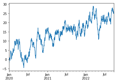
0x0D 作图 Plotting
ts = pd.Series(np.random.randn(1000), index=pd.date_range('1/1/2020', periods=1000))
ts = ts.cumsum()
ts.plot()
<matplotlib.axes._subplots.AxesSubplot at 0x250ccebcb70>
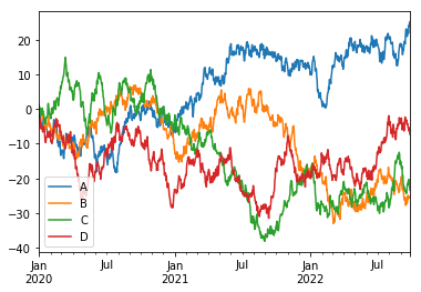
对于 DataFrame 而言,plot()方法是一种将所有带有标签的列进行绘制的简便方法。
df = pd.DataFrame(np.random.randn(1000, 4), index=ts.index,
                  columns=['A', 'B', 'C', 'D'])
# print(df)
df = df.cumsum()
plt.figure()
df.plot()
plt.legend(loc='best')
<matplotlib.legend.Legend at 0x250ce7620b8>
<Figure size 432x288 with 0 Axes>
ts.indexDatetimeIndex(['2020-01-01', '2020-01-02', '2020-01-03', '2020-01-04',
'2020-01-05', '2020-01-06', '2020-01-07', '2020-01-08',
'2020-01-09', '2020-01-10',
...
'2022-09-17', '2022-09-18', '2022-09-19', '2022-09-20',
'2022-09-21', '2022-09-22', '2022-09-23', '2022-09-24',
'2022-09-25', '2022-09-26'],
dtype='datetime64[ns]', length=1000, freq='D')
0x0E 导入导出数据 Getting Data In/Out
0x0E-1 CSV
写入 csv 文件
df.to_csv('foo.csv') # 保存在当前目录下从 csv 文件中导入数据
pd.read_csv('foo.csv')| Unnamed: 0 | A | B | C | D | |
|---|---|---|---|---|---|
| 0 | 2020-01-01 | -1.397481 | -0.453722 | 1.374079 | -2.095767 |
| 1 | 2020-01-02 | -1.363418 | 0.529293 | 0.178497 | -2.364989 |
| 2 | 2020-01-03 | -2.047267 | -0.333020 | 0.379978 | -2.628204 |
| 3 | 2020-01-04 | -2.305870 | -0.145598 | -0.232491 | -2.812290 |
| 4 | 2020-01-05 | -1.851390 | -1.378215 | -1.202399 | -4.574516 |
| 5 | 2020-01-06 | -3.438928 | -0.779975 | -1.864979 | -5.666847 |
| 6 | 2020-01-07 | -4.201270 | -0.827366 | -0.796513 | -5.267628 |
| 7 | 2020-01-08 | -5.682762 | -1.009404 | -0.760801 | -4.696243 |
| 8 | 2020-01-09 | -4.362126 | -0.768552 | -0.747517 | -5.562345 |
| 9 | 2020-01-10 | -5.226357 | -1.791920 | 0.290504 | -5.214061 |
| 10 | 2020-01-11 | -4.429691 | -2.026951 | -0.821212 | -6.621030 |
| 11 | 2020-01-12 | -4.222744 | -2.875169 | -0.654313 | -5.926621 |
| 12 | 2020-01-13 | -2.413314 | -3.329878 | -1.595397 | -5.585677 |
| 13 | 2020-01-14 | -2.769944 | -3.536045 | -1.463671 | -5.098753 |
| 14 | 2020-01-15 | -3.599683 | -4.973067 | -3.859425 | -5.823875 |
| 15 | 2020-01-16 | -3.486154 | -4.792330 | -2.866047 | -6.312086 |
| 16 | 2020-01-17 | -4.232714 | -5.082053 | -3.572924 | -8.478300 |
| 17 | 2020-01-18 | -5.346857 | -5.787422 | -4.313125 | -8.595854 |
| 18 | 2020-01-19 | -5.720494 | -5.620498 | -3.699862 | -9.678113 |
| 19 | 2020-01-20 | -5.264735 | -4.938944 | -2.354040 | -8.942524 |
| 20 | 2020-01-21 | -5.407854 | -5.379811 | -2.284447 | -8.068545 |
| 21 | 2020-01-22 | -5.793401 | -5.501279 | -2.254013 | -7.997644 |
| 22 | 2020-01-23 | -6.796539 | -4.692782 | -2.330458 | -7.449650 |
| 23 | 2020-01-24 | -7.502072 | -4.085084 | -1.810495 | -6.540544 |
| 24 | 2020-01-25 | -7.639024 | -3.791416 | 1.214301 | -7.599166 |
| 25 | 2020-01-26 | -7.783544 | -2.180918 | 1.628560 | -7.928116 |
| 26 | 2020-01-27 | -7.673699 | -3.485888 | 0.640970 | -8.124872 |
| 27 | 2020-01-28 | -7.435098 | -4.480212 | -0.409425 | -7.943383 |
| 28 | 2020-01-29 | -6.843557 | -5.069680 | -1.650871 | -7.311741 |
| 29 | 2020-01-30 | -7.647267 | -4.115332 | -1.558887 | -6.308304 |
| ... | ... | ... | ... | ... | ... |
| 970 | 2022-08-28 | 17.157914 | -23.306973 | -12.461653 | -2.478731 |
| 971 | 2022-08-29 | 18.207251 | -23.725280 | -12.912440 | -2.664828 |
| 972 | 2022-08-30 | 17.968302 | -21.485150 | -15.044877 | -4.034060 |
| 973 | 2022-08-31 | 18.933869 | -21.587237 | -16.046081 | -4.014128 |
| 974 | 2022-09-01 | 18.337284 | -21.451739 | -15.028398 | -4.147177 |
| 975 | 2022-09-02 | 18.783912 | -21.096423 | -15.506137 | -3.858413 |
| 976 | 2022-09-03 | 18.828378 | -19.514168 | -16.924864 | -2.559397 |
| 977 | 2022-09-04 | 18.570511 | -21.482747 | -17.147155 | -4.267082 |
| 978 | 2022-09-05 | 17.212119 | -22.331837 | -16.496095 | -5.990857 |
| 979 | 2022-09-06 | 15.726498 | -23.219830 | -19.321023 | -5.281962 |
| 980 | 2022-09-07 | 16.053999 | -22.681168 | -19.139536 | -5.587482 |
| 981 | 2022-09-08 | 17.335456 | -23.320514 | -21.271891 | -4.048170 |
| 982 | 2022-09-09 | 16.925567 | -24.175782 | -22.318101 | -4.890968 |
| 983 | 2022-09-10 | 18.652048 | -25.436089 | -22.213175 | -6.330027 |
| 984 | 2022-09-11 | 19.535978 | -25.673818 | -23.064392 | -5.673334 |
| 985 | 2022-09-12 | 19.632355 | -26.369119 | -22.953900 | -3.463010 |
| 986 | 2022-09-13 | 18.792587 | -25.430236 | -23.672206 | -2.292810 |
| 987 | 2022-09-14 | 21.200064 | -26.299390 | -23.567706 | -2.753986 |
| 988 | 2022-09-15 | 22.890536 | -27.813985 | -23.938164 | -3.195772 |
| 989 | 2022-09-16 | 23.138447 | -25.855344 | -24.390078 | -3.612660 |
| 990 | 2022-09-17 | 23.163567 | -26.157774 | -24.309178 | -3.155928 |
| 991 | 2022-09-18 | 20.973996 | -27.319631 | -22.948785 | -4.487101 |
| 992 | 2022-09-19 | 21.090756 | -26.712847 | -21.722990 | -4.110810 |
| 993 | 2022-09-20 | 21.848391 | -25.018472 | -21.850579 | -4.360523 |
| 994 | 2022-09-21 | 22.898217 | -26.005364 | -20.914269 | -5.357187 |
| 995 | 2022-09-22 | 21.978310 | -25.001244 | -20.881626 | -5.606849 |
| 996 | 2022-09-23 | 24.132628 | -25.692639 | -20.310265 | -6.258977 |
| 997 | 2022-09-24 | 23.777794 | -25.485527 | -21.305882 | -5.330284 |
| 998 | 2022-09-25 | 25.105611 | -25.485135 | -22.407657 | -6.600228 |
| 999 | 2022-09-26 | 25.207099 | -25.512208 | -23.434955 | -7.275999 |
1000 rows × 5 columns
0x0E-2 HDF5
写入 HDF5 存储
df.to_hdf('foo.h5','df')从 HDF5 存储中读取数据
pd.read_hdf('foo.h5','df')| A | B | C | D | |
|---|---|---|---|---|
| 2020-01-01 | -1.397481 | -0.453722 | 1.374079 | -2.095767 |
| 2020-01-02 | -1.363418 | 0.529293 | 0.178497 | -2.364989 |
| 2020-01-03 | -2.047267 | -0.333020 | 0.379978 | -2.628204 |
| 2020-01-04 | -2.305870 | -0.145598 | -0.232491 | -2.812290 |
| 2020-01-05 | -1.851390 | -1.378215 | -1.202399 | -4.574516 |
| 2020-01-06 | -3.438928 | -0.779975 | -1.864979 | -5.666847 |
| 2020-01-07 | -4.201270 | -0.827366 | -0.796513 | -5.267628 |
| 2020-01-08 | -5.682762 | -1.009404 | -0.760801 | -4.696243 |
| 2020-01-09 | -4.362126 | -0.768552 | -0.747517 | -5.562345 |
| 2020-01-10 | -5.226357 | -1.791920 | 0.290504 | -5.214061 |
| 2020-01-11 | -4.429691 | -2.026951 | -0.821212 | -6.621030 |
| 2020-01-12 | -4.222744 | -2.875169 | -0.654313 | -5.926621 |
| 2020-01-13 | -2.413314 | -3.329878 | -1.595397 | -5.585677 |
| 2020-01-14 | -2.769944 | -3.536045 | -1.463671 | -5.098753 |
| 2020-01-15 | -3.599683 | -4.973067 | -3.859425 | -5.823875 |
| 2020-01-16 | -3.486154 | -4.792330 | -2.866047 | -6.312086 |
| 2020-01-17 | -4.232714 | -5.082053 | -3.572924 | -8.478300 |
| 2020-01-18 | -5.346857 | -5.787422 | -4.313125 | -8.595854 |
| 2020-01-19 | -5.720494 | -5.620498 | -3.699862 | -9.678113 |
| 2020-01-20 | -5.264735 | -4.938944 | -2.354040 | -8.942524 |
| 2020-01-21 | -5.407854 | -5.379811 | -2.284447 | -8.068545 |
| 2020-01-22 | -5.793401 | -5.501279 | -2.254013 | -7.997644 |
| 2020-01-23 | -6.796539 | -4.692782 | -2.330458 | -7.449650 |
| 2020-01-24 | -7.502072 | -4.085084 | -1.810495 | -6.540544 |
| 2020-01-25 | -7.639024 | -3.791416 | 1.214301 | -7.599166 |
| 2020-01-26 | -7.783544 | -2.180918 | 1.628560 | -7.928116 |
| 2020-01-27 | -7.673699 | -3.485888 | 0.640970 | -8.124872 |
| 2020-01-28 | -7.435098 | -4.480212 | -0.409425 | -7.943383 |
| 2020-01-29 | -6.843557 | -5.069680 | -1.650871 | -7.311741 |
| 2020-01-30 | -7.647267 | -4.115332 | -1.558887 | -6.308304 |
| ... | ... | ... | ... | ... |
| 2022-08-28 | 17.157914 | -23.306973 | -12.461653 | -2.478731 |
| 2022-08-29 | 18.207251 | -23.725280 | -12.912440 | -2.664828 |
| 2022-08-30 | 17.968302 | -21.485150 | -15.044877 | -4.034060 |
| 2022-08-31 | 18.933869 | -21.587237 | -16.046081 | -4.014128 |
| 2022-09-01 | 18.337284 | -21.451739 | -15.028398 | -4.147177 |
| 2022-09-02 | 18.783912 | -21.096423 | -15.506137 | -3.858413 |
| 2022-09-03 | 18.828378 | -19.514168 | -16.924864 | -2.559397 |
| 2022-09-04 | 18.570511 | -21.482747 | -17.147155 | -4.267082 |
| 2022-09-05 | 17.212119 | -22.331837 | -16.496095 | -5.990857 |
| 2022-09-06 | 15.726498 | -23.219830 | -19.321023 | -5.281962 |
| 2022-09-07 | 16.053999 | -22.681168 | -19.139536 | -5.587482 |
| 2022-09-08 | 17.335456 | -23.320514 | -21.271891 | -4.048170 |
| 2022-09-09 | 16.925567 | -24.175782 | -22.318101 | -4.890968 |
| 2022-09-10 | 18.652048 | -25.436089 | -22.213175 | -6.330027 |
| 2022-09-11 | 19.535978 | -25.673818 | -23.064392 | -5.673334 |
| 2022-09-12 | 19.632355 | -26.369119 | -22.953900 | -3.463010 |
| 2022-09-13 | 18.792587 | -25.430236 | -23.672206 | -2.292810 |
| 2022-09-14 | 21.200064 | -26.299390 | -23.567706 | -2.753986 |
| 2022-09-15 | 22.890536 | -27.813985 | -23.938164 | -3.195772 |
| 2022-09-16 | 23.138447 | -25.855344 | -24.390078 | -3.612660 |
| 2022-09-17 | 23.163567 | -26.157774 | -24.309178 | -3.155928 |
| 2022-09-18 | 20.973996 | -27.319631 | -22.948785 | -4.487101 |
| 2022-09-19 | 21.090756 | -26.712847 | -21.722990 | -4.110810 |
| 2022-09-20 | 21.848391 | -25.018472 | -21.850579 | -4.360523 |
| 2022-09-21 | 22.898217 | -26.005364 | -20.914269 | -5.357187 |
| 2022-09-22 | 21.978310 | -25.001244 | -20.881626 | -5.606849 |
| 2022-09-23 | 24.132628 | -25.692639 | -20.310265 | -6.258977 |
| 2022-09-24 | 23.777794 | -25.485527 | -21.305882 | -5.330284 |
| 2022-09-25 | 25.105611 | -25.485135 | -22.407657 | -6.600228 |
| 2022-09-26 | 25.207099 | -25.512208 | -23.434955 | -7.275999 |
1000 rows × 4 columns
0x0E-3 Excel
看网上说,相对于 xlwt、xlrd 之类的库,用 pandas 来对 excel 进行数据处理和分析挺不错的,正好最近也想试试呢。
写入 Excel
df.to_excel('foo.xlsx', sheet_name='Sheet1')从 excel 中读取数据
pd.read_excel('foo.xlsx', 'Sheet1', index_col=None, na_values=['NA'])| Unnamed: 0 | A | B | C | D | |
|---|---|---|---|---|---|
| 0 | 2020-01-01 | -1.397481 | -0.453722 | 1.374079 | -2.095767 |
| 1 | 2020-01-02 | -1.363418 | 0.529293 | 0.178497 | -2.364989 |
| 2 | 2020-01-03 | -2.047267 | -0.333020 | 0.379978 | -2.628204 |
| 3 | 2020-01-04 | -2.305870 | -0.145598 | -0.232491 | -2.812290 |
| 4 | 2020-01-05 | -1.851390 | -1.378215 | -1.202399 | -4.574516 |
| 5 | 2020-01-06 | -3.438928 | -0.779975 | -1.864979 | -5.666847 |
| 6 | 2020-01-07 | -4.201270 | -0.827366 | -0.796513 | -5.267628 |
| 7 | 2020-01-08 | -5.682762 | -1.009404 | -0.760801 | -4.696243 |
| 8 | 2020-01-09 | -4.362126 | -0.768552 | -0.747517 | -5.562345 |
| 9 | 2020-01-10 | -5.226357 | -1.791920 | 0.290504 | -5.214061 |
| 10 | 2020-01-11 | -4.429691 | -2.026951 | -0.821212 | -6.621030 |
| 11 | 2020-01-12 | -4.222744 | -2.875169 | -0.654313 | -5.926621 |
| 12 | 2020-01-13 | -2.413314 | -3.329878 | -1.595397 | -5.585677 |
| 13 | 2020-01-14 | -2.769944 | -3.536045 | -1.463671 | -5.098753 |
| 14 | 2020-01-15 | -3.599683 | -4.973067 | -3.859425 | -5.823875 |
| 15 | 2020-01-16 | -3.486154 | -4.792330 | -2.866047 | -6.312086 |
| 16 | 2020-01-17 | -4.232714 | -5.082053 | -3.572924 | -8.478300 |
| 17 | 2020-01-18 | -5.346857 | -5.787422 | -4.313125 | -8.595854 |
| 18 | 2020-01-19 | -5.720494 | -5.620498 | -3.699862 | -9.678113 |
| 19 | 2020-01-20 | -5.264735 | -4.938944 | -2.354040 | -8.942524 |
| 20 | 2020-01-21 | -5.407854 | -5.379811 | -2.284447 | -8.068545 |
| 21 | 2020-01-22 | -5.793401 | -5.501279 | -2.254013 | -7.997644 |
| 22 | 2020-01-23 | -6.796539 | -4.692782 | -2.330458 | -7.449650 |
| 23 | 2020-01-24 | -7.502072 | -4.085084 | -1.810495 | -6.540544 |
| 24 | 2020-01-25 | -7.639024 | -3.791416 | 1.214301 | -7.599166 |
| 25 | 2020-01-26 | -7.783544 | -2.180918 | 1.628560 | -7.928116 |
| 26 | 2020-01-27 | -7.673699 | -3.485888 | 0.640970 | -8.124872 |
| 27 | 2020-01-28 | -7.435098 | -4.480212 | -0.409425 | -7.943383 |
| 28 | 2020-01-29 | -6.843557 | -5.069680 | -1.650871 | -7.311741 |
| 29 | 2020-01-30 | -7.647267 | -4.115332 | -1.558887 | -6.308304 |
| ... | ... | ... | ... | ... | ... |
| 970 | 2022-08-28 | 17.157914 | -23.306973 | -12.461653 | -2.478731 |
| 971 | 2022-08-29 | 18.207251 | -23.725280 | -12.912440 | -2.664828 |
| 972 | 2022-08-30 | 17.968302 | -21.485150 | -15.044877 | -4.034060 |
| 973 | 2022-08-31 | 18.933869 | -21.587237 | -16.046081 | -4.014128 |
| 974 | 2022-09-01 | 18.337284 | -21.451739 | -15.028398 | -4.147177 |
| 975 | 2022-09-02 | 18.783912 | -21.096423 | -15.506137 | -3.858413 |
| 976 | 2022-09-03 | 18.828378 | -19.514168 | -16.924864 | -2.559397 |
| 977 | 2022-09-04 | 18.570511 | -21.482747 | -17.147155 | -4.267082 |
| 978 | 2022-09-05 | 17.212119 | -22.331837 | -16.496095 | -5.990857 |
| 979 | 2022-09-06 | 15.726498 | -23.219830 | -19.321023 | -5.281962 |
| 980 | 2022-09-07 | 16.053999 | -22.681168 | -19.139536 | -5.587482 |
| 981 | 2022-09-08 | 17.335456 | -23.320514 | -21.271891 | -4.048170 |
| 982 | 2022-09-09 | 16.925567 | -24.175782 | -22.318101 | -4.890968 |
| 983 | 2022-09-10 | 18.652048 | -25.436089 | -22.213175 | -6.330027 |
| 984 | 2022-09-11 | 19.535978 | -25.673818 | -23.064392 | -5.673334 |
| 985 | 2022-09-12 | 19.632355 | -26.369119 | -22.953900 | -3.463010 |
| 986 | 2022-09-13 | 18.792587 | -25.430236 | -23.672206 | -2.292810 |
| 987 | 2022-09-14 | 21.200064 | -26.299390 | -23.567706 | -2.753986 |
| 988 | 2022-09-15 | 22.890536 | -27.813985 | -23.938164 | -3.195772 |
| 989 | 2022-09-16 | 23.138447 | -25.855344 | -24.390078 | -3.612660 |
| 990 | 2022-09-17 | 23.163567 | -26.157774 | -24.309178 | -3.155928 |
| 991 | 2022-09-18 | 20.973996 | -27.319631 | -22.948785 | -4.487101 |
| 992 | 2022-09-19 | 21.090756 | -26.712847 | -21.722990 | -4.110810 |
| 993 | 2022-09-20 | 21.848391 | -25.018472 | -21.850579 | -4.360523 |
| 994 | 2022-09-21 | 22.898217 | -26.005364 | -20.914269 | -5.357187 |
| 995 | 2022-09-22 | 21.978310 | -25.001244 | -20.881626 | -5.606849 |
| 996 | 2022-09-23 | 24.132628 | -25.692639 | -20.310265 | -6.258977 |
| 997 | 2022-09-24 | 23.777794 | -25.485527 | -21.305882 | -5.330284 |
| 998 | 2022-09-25 | 25.105611 | -25.485135 | -22.407657 | -6.600228 |
| 999 | 2022-09-26 | 25.207099 | -25.512208 | -23.434955 | -7.275999 |
1000 rows × 5 columns
0x0F 陷阱 Gotchas
如果你在运行中看到例如下面的异常。
if pd.Series([False, True, False]):
    print("I was true")
---------------------------------------------------------------------------
ValueError Traceback (most recent call last)
<ipython-input-304-5c782b38cd2f> in <module>
----> 1 if pd.Series([False, True, False]):
2 print("I was true")
D:\Programs\Anaconda\lib\site-packages\pandas\core\generic.py in __nonzero__(self)
1476 raise ValueError("The truth value of a {0} is ambiguous. "
1477 "Use a.empty, a.bool(), a.item(), a.any() or a.all()."
-> 1478 .format(self.__class__.__name__))
1479
1480 __bool__ = __nonzero__
ValueError: The truth value of a Series is ambiguous. Use a.empty, a.bool(), a.item(), a.any() or a.all().
可以参考 Comparisons 这里来寻求解释和下一步的方案。
也可以参考 Comparisons。
(上面都是官方的文档地址)
(官方文档到这里就结束了)
0x10 小结
关于选取:
- 选择整行/整列,或多个整行/多个整列的数据,可以用
df[]、df.loc[]、df.iloc[]这三种用法。 - 区域选取,分为标签索引和整数索引
- 标签索引:
df.loc[] - 整数索引:
df.iloc[]
- 标签索引:
- 选取单元格:
df.at[]、df.iat[]、df.loc[]、df.iloc[]都可以,要注意参数。df[]不行! - 关于选取的返回值:
- 返回值包括单行多列或多行单列时,返回值为 Series 对象
- 返回值包括多行多列时,返回值为 DataFrame 对象
- 返回值仅为一个单元格(单行单列)时,返回值为(可能是 numpy 的)基本数据类型,例如 str, float64, int64 等
df[]因为不能精确到单元格,所以返回值一定 DataFrame 或 Series 对象
- 当使用 DataFrame 的默认索引(整数索引)时,整数索引即为标签索引。
其实 pandas 还有很多有用的 API 这里面还没介绍,后面有空再慢慢了解呢。
做项目的时候看看别人做过的实例,再深入看看相关的 API 好了。
大概就这些内容了吧。
(溜了溜了
20200418 更新:
Jupyter Notebook 文档 (.ipynb) 放到 GitHub 上了,详见这里:https://github.com/miaotony/DataScience/blob/master/10_Minutes_to_pandas.ipynb
下载文档的话 戳这里(CDN,推荐) 呢!或者 也可以戳这里(GitHub raw)!
0xFF References & Extensive Reading
[python数据分析之pandas数据选取:df] df.loc[] df.iloc[] df.ix[] df.at[] df.iat[]
从Excel到Python:最常用的36个Pandas函数!
etc.


